1
2
3


import numpy as np
import pandas as pd
import matplotlib.pyplot as plt

1
2


A = np.eye(5)
A

array([[1., 0., 0., 0., 0.],
       [0., 1., 0., 0., 0.],
       [0., 0., 1., 0., 0.],
       [0., 0., 0., 1., 0.],
       [0., 0., 0., 0., 1.]])

单变量的线性回归

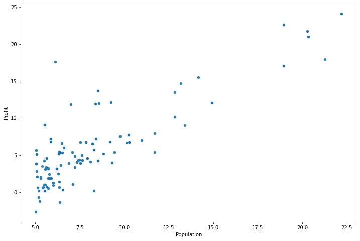
整个2的部分需要根据城市人口数量，预测开小吃店的利润数据在ex1data1.txt里，第一列是城市人口数量，第二列是该城市小吃店利润。

1
2
3


path =  'ex1data1.txt'
data = pd.read_csv(path, header=None, names=['Population', 'Profit'])
data.head()

	Population	Profit
0	6.1101	17.5920
1	5.5277	9.1302
2	8.5186	13.6620
3	7.0032	11.8540
4	5.8598	6.8233

1
2


data.plot(kind='scatter',x='Population',y='Profit', figsize=(12,8))
plt.show()

梯度下降

这个部分你需要在现有数据集上，训练线性回归的参数θ

1
2
3
4


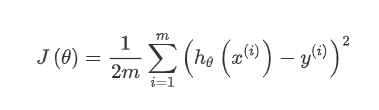
def computeCost(X, y, theta):
    inner = np.power(((X * theta.T) - y), 2)
    return np.sum(inner) / (2 * len(X))
#代价函数

数据前面已经读取完毕，我们要为加入一列x，用于更新θ0，然后我们将θ初始化为0，学习率初始化为0.01，迭代次数为1500次

1

data.insert(0, 'Ones', 1)

1
2
3
4


# 初始化X和y
cols = data.shape[1]
X = data.iloc[:,:-1]#X是data里的除最后列
y = data.iloc[:,cols-1:cols]#y是data最后一列

1

X.head()#head()观察前五行

	Ones	Population
0	1	6.1101
1	1	5.5277
2	1	8.5186
3	1	7.0032
4	1	5.8598

1

y.head()

	Profit
0	17.5920
1	9.1302
2	13.6620
3	11.8540
4	6.8233

代价函数是应该是numpy矩阵，所以我们需要转换X和Y，然后才能使用它们。我们还需要初始化theta。

1
2
3


X = np.matrix(X.values)
y = np.matrix(y.values)
theta = np.matrix(np.array([0,0]))

1
2


X.shape, theta.shape, y.shape
#shape矩阵的维度

((97, 2), (1, 2), (97, 1))

计算代价函数 (theta初始值为0)

1

computeCost(X, y, theta)

32.072733877455676

梯度下降（未写）

 1
 2
 3
 4
 5
 6
 7
 8
 9
10
11
12
13
14
15
16
17


def gradientDescent(X, y, theta, alpha, iters):
    temp = np.matrix(np.zeros(theta.shape))
    parameters = int(theta.ravel().shape[1])
    cost = np.zeros(iters)
    
    for i in range(iters):
        error = (X * theta.T) - y
        
        for j in range(parameters):
            term = np.multiply(error, X[:,j])
            temp[0,j] = theta[0,j] - ((alpha / len(X)) * np.sum(term))
            
        theta = temp
        cost[i] = computeCost(X, y, theta)
        
    return theta, cost
#这个部分实现了Ѳ的更新

1
2


alpha = 0.01
iters = 1500

1
2


g, cost = gradientDescent(X, y, theta, alpha, iters)
g

matrix([[-3.63029144,  1.16636235]])

1
2
3
4
5


predict1 = [1,3.5]*g.T
print("predict1:",predict1)
predict2 = [1,7]*g.T
print("predict2:",predict2)
#预测35000和70000城市规模的小吃摊利润

predict1: [[0.45197679]]
predict2: [[4.53424501]]

 1
 2
 3
 4
 5
 6
 7
 8
 9
10
11
12


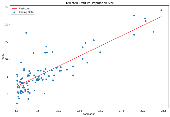
x = np.linspace(data.Population.min(), data.Population.max(), 100)
f = g[0, 0] + (g[0, 1] * x)

fig, ax = plt.subplots(figsize=(12,8))
ax.plot(x, f, 'r', label='Prediction')
ax.scatter(data.Population, data.Profit, label='Traning Data')
ax.legend(loc=2)
ax.set_xlabel('Population')
ax.set_ylabel('Profit')
ax.set_title('Predicted Profit vs. Population Size')
plt.show()
#原始数据以及拟合的直线

ex1线性回归

Contents

单变量的线性回归

梯度下降