Pseudo Labelling
Contents
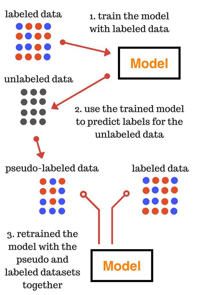
伪标签
半监督学习,即使用标签数据(受监督的学习)和不加标签的数据(无监督的学习)。

我们不需要手动标记不加标签的数据,而是根据标签的数据给出近似的标签。
-
第一步:使用标签数据训练模型
-
第二步:使用训练的模型为不加标签的数据预测标签
-
第三步:同时使用pseudo和标签数据集重新训练模型
在第三步中训练的最终模型用于对测试数据的最终预测。
我们将使用来自AV数据处理平台的大市场销售(Big Mart Sales)问题。因此,让我们从下载数据部分中的训练和测试文件开始。
导入库
|
|
|
|
| Item_Identifier | Item_Weight | Item_Fat_Content | Item_Visibility | Item_Type | Item_MRP | Outlet_Identifier | Outlet_Establishment_Year | Outlet_Size | Outlet_Location_Type | Outlet_Type | Item_Outlet_Sales | |
|---|---|---|---|---|---|---|---|---|---|---|---|---|
| 0 | FDA15 | 9.30 | Low Fat | 0.016047 | Dairy | 249.8092 | OUT049 | 1999 | Medium | Tier 1 | Supermarket Type1 | 3735.1380 |
| 1 | DRC01 | 5.92 | Regular | 0.019278 | Soft Drinks | 48.2692 | OUT018 | 2009 | Medium | Tier 3 | Supermarket Type2 | 443.4228 |
| 2 | FDN15 | 17.50 | Low Fat | 0.016760 | Meat | 141.6180 | OUT049 | 1999 | Medium | Tier 1 | Supermarket Type1 | 2097.2700 |
| 3 | FDX07 | 19.20 | Regular | 0.000000 | Fruits and Vegetables | 182.0950 | OUT010 | 1998 | NaN | Tier 3 | Grocery Store | 732.3800 |
| 4 | NCD19 | 8.93 | Low Fat | 0.000000 | Household | 53.8614 | OUT013 | 1987 | High | Tier 3 | Supermarket Type1 | 994.7052 |
看一下我们下载的训练和测试文件,并进行一些基本的预处理,以形成模型。
|
|
| Item_Weight | Item_Fat_Content | Item_Visibility | Item_MRP | Outlet_Establishment_Year | Outlet_Size | Outlet_Location_Type | Outlet_Type | |
|---|---|---|---|---|---|---|---|---|
| 0 | 9.30 | 0 | 0.016047 | 249.8092 | 1999 | 1 | 0 | 1 |
| 1 | 5.92 | 1 | 0.019278 | 48.2692 | 2009 | 1 | 2 | 2 |
| 2 | 17.50 | 0 | 0.016760 | 141.6180 | 1999 | 1 | 0 | 1 |
| 3 | 19.20 | 1 | 0.000000 | 182.0950 | 1998 | 2 | 2 | 0 |
| 4 | 8.93 | 0 | 0.000000 | 53.8614 | 1987 | 0 | 2 | 1 |
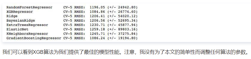
从不同的监督学习算法开始,让我们来看看哪一种算法给了我们最好的结果。
|
|
|
|
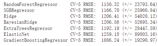
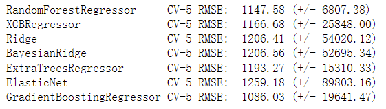
!!!和原文跑出不一样。。GradientBoostingRegressor算法最好
|
|
|
|
现在,让我们来实现伪标签,为了这个目的,我将使用测试数据作为不加标签的数据。
|
|
现在,让我们来检查一下数据集上的伪标签的结果
|
|
|
|
|
|
|
|

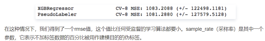
在这种情况下,我们得到了一个rmse值,这个值比任何受监督的学习算法都要小。
sample_rate(采样率)是其中一个参数,它表示不加标签数据的百分比被用作建模目的的伪标签。
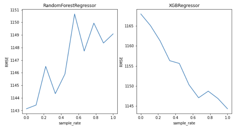
因此,让我们检查一下采样率对伪标签性能的依赖性。
采样率的依赖
为了找出样本率对伪标签性能的依赖,让我们在这两者之间画一个图。在这里,我只使用了两种算法来表示对时间约束(time constraint)的依赖,但你也可以尝试其他算法。
|
|
https://cloud.tencent.com/developer/article/1050723
https://www.analyticsvidhya.com/blog/2017/09/pseudo-labelling-semi-supervised-learning-technique/
https://github.com/shubhamjn1/Pseudo-Labelling---A-Semi-supervised-learning-technique
Author kong
LastMod 2022-01-06